并行计算简介 Introduction: Parallel Computing
This article is based on the teaching material of University of Melbourne COMP90025, material by Dr. Aaron Harwood.
RAM and PRAM Model
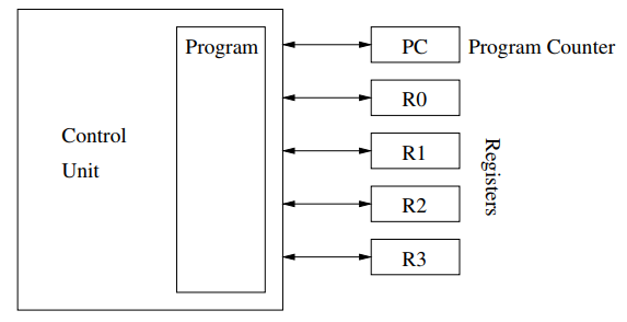
RAM (随机存取机) stands for Random Access Machine, which is a simple model of computation. A program in a RAM runs according the program counter, and the operation (in the program) is translated to a constant number of instructions. It is called “random” because the time taken to access the memory is constant over all addresses.
在RAM中,一个程序中的每个语句都会被编译成不同的指令(instructions),但是指令的数量与算法本身的复杂度是没有关系的。也就是说,假设输入由\(n\)变成\(n^2\),编译出来指令的数量不会变化。另外,在RAM中,访问内存中的任意位置所需要的时间是一致的,内存中任意位置存放的信息的大小也是一致的。
 RAM slide
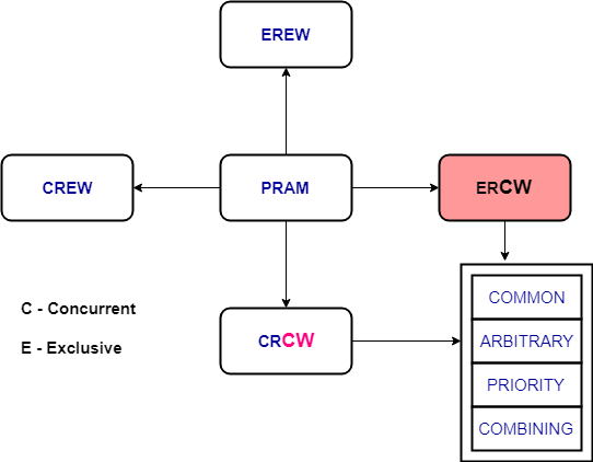
PRAM stands for Parallel Random Access Machine. According to Karp and Ramachandran (1988) which assumes that each processor has random access in unit time to any cell of a global memory. This ideal model permits separation of parallel computation and issues of interprocessor communication. A [slide] (/myblog/assets/pram.pdf) from Kent State University is useful for further understand the concepts.
简单来说,PRAM是一个用于将处理器之间的数据传递和并行算法本身分隔开的理想化模型, PRAM中的每一个node都是符合RAM模型的。一般来说,PRAM的机器是不可能制造出来的(因为统一读写“共享内存“的速度基本是无法实现的)。还有一点是,一般会假设能用的处理器(processor)的个数等于问题的大小,因为将适用于更多处理器的算法应用到少量处理器上是不难做到(而且少处理器个数(p2)能整除更多处理器(p1)时,work是相等的),但反过来就很难。
Metrics on PRAM Model
input size \(n\) , number of processor \(p(n)\), number of sequential steps (sequential time complexity) \(T(n)\), number of parallel steps (each step \(t_i\) contains \(x_i\) operations ) \(t(n)\).
work size \(w(n)\ =\ t(n)\ *\ p(n)\)
total number of operations \(size(n)\ =\ \sum_{i=1}^{t(n)} x_i\)
speed up \(S(p(n))\ =\ \frac{T(n)}{t_p(n)}\)
efficiency \(E(p(n))\ =\ \frac{S(p(n))}{p(n)}\)
Optimal if: \(t(n)\ =\ O(log^c(n))\) for some constant \(c\) (poly-logarithmic) and \(w(n)\ =\ O(T(n))\)
efficient if: \(t(n)\ =\ O(log^c(n))\) for some constant \(c\) and \(w(n)\ =\ T(n) * O(log^cn)\)
Brent’s Principle
Brent’s principle can be used to infer the best running time for a parallel algorithm that runs with a given size. For one parallel step \(t_i\),
\(t_i\ =\ \lceil{\frac{x_i}{p}}\rceil\) <= \(\frac{x_i}{p}\ +\ \frac{p-1}{p}\)
To sum up all steps,
\(\sum_{i=1}^{t}t_i\) = \(\frac{x}{p}\) + \(t\) - \(\frac{t}{p}\) = \(t\) + \(\frac{x-t}{p}\)
Notice that in the equation above, \(t\) is the total number of parallel steps (parallel time complexity), which is \(t(n)\).
Amdahl’s Law Amdahl’s Law is one way of predicting the maximum achievable speedup for a given program, where \(f\) is the fraction (percentage, like 40%) of sequential steps.
\[S(p)\ =\ \frac{p}{1+(p-1)f}\]Gustafson’s Law Similar to Amdahl’s law,
\[S(p)\ =\ p+(1-p)f\]